Tutorial
Download and Explore NEON Data
Last Updated: Nov 28, 2023
This tutorial covers downloading NEON data, using the Data Portal and the neonUtilities R package, as well as basic instruction in beginning to explore and work with the downloaded data, including guidance in navigating data documentation. We will explore data of 3 different types, and make a simple figure from each.
NEON data
There are 3 basic categories of NEON data:
- Remote sensing (AOP) - Data collected by the airborne observation platform, e.g. LIDAR, surface reflectance
- Observational (OS) - Data collected by a human in the field, or in an analytical laboratory, e.g. beetle identification, foliar isotopes
- Instrumentation (IS) - Data collected by an automated, streaming sensor, e.g. net radiation, soil carbon dioxide. This category also includes the eddy covariance (EC) data, which are processed and structured in a unique way, distinct from other instrumentation data (see Tutorial for EC data for details).
This lesson covers all three types of data. The download procedures are similar for all types, but data navigation differs significantly by type.
Objectives
After completing this activity, you will be able to:
- Download NEON data using the neonUtilities package.
- Understand downloaded data sets and load them into R for analyses.
Things You’ll Need To Complete This Tutorial
To complete this tutorial you will need the most current version of R and, preferably, RStudio loaded on your computer.
Install R Packages
- neonUtilities: Basic functions for accessing NEON data
- neonOS: Functions for common data wrangling needs for NEON observational data
- terra: Spatial data package; needed for remote sensing data
These packages can be installed from CRAN:
install.packages("neonUtilities")

install.packages("neonOS")

install.packages("terra")
Additional Resources
- Tutorial for using neonUtilities from a Python environment.
- GitHub repository for neonUtilities
- neonUtilities cheat sheet. A quick reference guide for users.
Getting started: Download data from the Portal and load packages
Go to the NEON Data Portal and download some data! To follow the tutorial exactly, download Photosynthetically active radiation (PAR) (DP1.00024.001) data from September-November 2019 at Wind River Experimental Forest (WREF). The downloaded file should be a zip file named NEON_par.zip.
If you prefer to explore a different data product, you can still follow this tutorial. But it will be easier to understand the steps in the tutorial, particularly the data navigation, if you choose a sensor data product for this section.
Once you've downloaded a zip file of data from the portal, switch over to R and load all the packages installed above.
# load packages

library(neonUtilities)

library(neonOS)

library(terra)


# Set global option to NOT convert all character variables to factors.

# If you are working in R version 4 or higher (recommended), this is

# already the default setting.

options(stringsAsFactors=F)
Stack the downloaded data files: stackByTable()
The stackByTable() function will unzip and join the files in the
downloaded zip file.
# Modify the file path to match the path to your zip file

stackByTable("~/Downloads/NEON_par.zip")
In the same directory as the zipped file, you should now have an unzipped folder of the same name. When you open this you will see a new folder called stackedFiles, which should contain at least seven files: PARPAR_30min.csv, PARPAR_1min.csv, sensor_positions.csv, variables_00024.csv, readme_00024.txt, issueLog_00024.csv, and citation_00024_RELEASE-202X.txt.
Navigate data downloads: IS
Let's start with a brief description of each file. This set of files is typical of a NEON IS data product.
- PARPAR_30min.csv: PAR data at 30-minute averaging intervals
- PARPAR_1min.csv: PAR data at 1-minute averaging intervals
- sensor_positions.csv: The physical location of each sensor collecting PAR measurements. There is a PAR sensor at each level of the WREF tower, and this table lets you connect the tower level index to the height of the sensor in meters.
- variables_00024.csv: Definitions and units for each data field in the PARPAR_#min tables.
- readme_00024.txt: Basic information about the PAR data product.
- issueLog_00024.csv: A record of known issues associated with PAR data.
- citation_00024_RELEASE-202X.txt: The citation to use when you publish a paper using these data, in BibTeX format.
We'll explore the 30-minute data. To read the file into R, use the function
readTableNEON(), which uses the variables file to assign data types to each
column of data:
par30 <- readTableNEON(
  dataFile="~/Downloads/NEON_par/stackedFiles/PARPAR_30min.csv",
  varFile="~/Downloads/NEON_par/stackedFiles/variables_00024.csv")

View(par30)
The first four columns are added by stackByTable() when it merges
files across sites, months, and tower heights. The column
publicationDate is the date-time stamp indicating when the data
were published, and the release column indicates which NEON data release
the data belong to. For more information about NEON data releases, see the
Data Product Revisions and Releases page.
Information about each data column can be found in the variables file:
parvar <- read.csv("~/Downloads/NEON_par/stackedFiles/variables_00024.csv")

View(parvar)
Here you can see definitions and units for each column of data.
Now that we know what we're looking at, let's plot PAR from the top tower level. We'll use the mean PAR from each averaging interval, and we can see from the sensor positions file that the vertical index 080 corresponds to the highest tower level. To explore the sensor positions data in more depth, see the spatial data tutorial.
plot(PARMean~startDateTime,
     data=par30[which(par30$verticalPosition=="080"),],
     type="l")
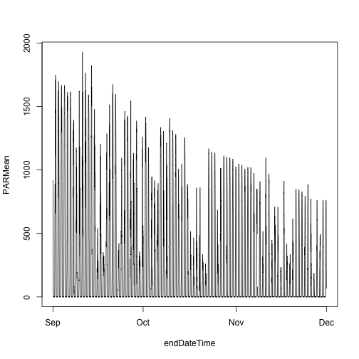
Looks good! The sun comes up and goes down every day, and some days are cloudy.
To see another layer of data, add PAR from a lower tower level to the plot.
plot(PARMean~startDateTime,
     data=par30[which(par30$verticalPosition=="080"),],
     type="l")


lines(PARMean~startDateTime,
     data=par30[which(par30$verticalPosition=="020"),],
     col="blue")
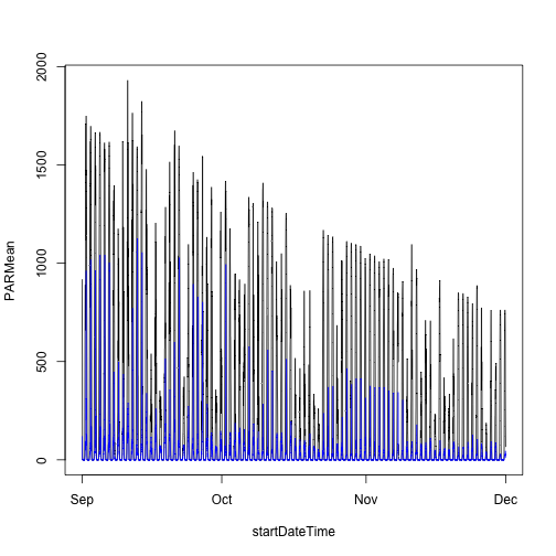
We can see there is a lot of light attenuation through the canopy.
Download files and load directly to R: loadByProduct()
At the start of this tutorial, we downloaded data from the NEON data portal.
NEON also provides an API, and the neonUtilities packages provides methods
for downloading programmatically in R.
The steps we carried out above - downloading from the portal, stacking the
downloaded files, and reading in to R - can all be carried out in one step by
the neonUtilities function loadByProduct().
To get the same PAR data we worked with above, we would run this line of code
using loadByProduct():
parlist <- loadByProduct(dpID="DP1.00024.001",
                         site="WREF",
                         startdate="2019-09",
                         enddate="2019-11")
The object returned by loadByProduct() is a named list. The objects in the
list are the same set of tables we ended with after stacking the data from
the portal above. You can see this by checking the names of the tables in
parlist:
names(parlist)

## [1] "citation_00024_RELEASE-2023" "issueLog_00024"              "PARPAR_1min"
## [4] "PARPAR_30min"                "readme_00024"                "sensor_positions_00024"
## [7] "variables_00024"
Now let's walk through the details of the inputs and options in
loadByProduct().
This function downloads data from the NEON API, merges the site-by-month files, and loads the resulting data tables into the R environment, assigning each data type to the appropriate R class. This is a popular choice for NEON data users because it ensures you're always working with the latest data, and it ends with ready-to-use tables in R. However, if you use it in a workflow you run repeatedly, keep in mind it will re-download the data every time. See below for suggestions on saving the data locally.
loadByProduct() works on most observational (OS) and sensor (IS) data,
but not on surface-atmosphere exchange (SAE) data, remote sensing (AOP)
data, and some of the data tables in the microbial data products. For
functions that download AOP data, see the final
section in this tutorial. For functions that work with SAE data, see
the NEON eddy flux data tutorial.
The inputs to loadByProduct() control which data to download and how
to manage the processing:
-
dpID: the data product ID, e.g. DP1.00002.001 -
site: defaults to "all", meaning all sites with available data; can be a vector of 4-letter NEON site codes, e.g.c("HARV","CPER","ABBY"). -
startdateandenddate: defaults to NA, meaning all dates with available data; or a date in the form YYYY-MM, e.g. 2017-06. Since NEON data are provided in month packages, finer scale querying is not available. Both start and end date are inclusive. -
package: either basic or expanded data package. Expanded data packages generally include additional information about data quality, such as chemical standards and quality flags. Not every data product has an expanded package; if the expanded package is requested but there isn't one, the basic package will be downloaded. -
timeIndex: defaults to "all", to download all data; or the number of minutes in the averaging interval. Only applicable to IS data. -
include.provisional: T or F: should Provisional data be included in the download? Defaults to F to return only Released data, which are citable by a DOI and do not change over time. Provisional data are subject to change. -
check.size: T or F: should the function pause before downloading data and warn you about the size of your download? Defaults to T; if you are using this function within a script or batch process you will want to set it to F. -
nCores: Number of cores to use for parallel processing. Defaults to 1, i.e. no parallelization. -
forceParallel: If the data volume to be processed does not meet minimum requirements to run in parallel, this overrides.
The dpID is the data product identifier of the data you want to
download. The DPID can be found on the
Explore Data Products page.
It will be in the form DP#.#####.###
To explore observational data, we'll download aquatic plant chemistry data (DP1.20063.001) from three lake sites: Prairie Lake (PRLA), Suggs Lake (SUGG), and Toolik Lake (TOOK).
apchem <- loadByProduct(dpID="DP1.20063.001",

                  site=c("PRLA","SUGG","TOOK"),

                  package="expanded", check.size=T)
Navigate data downloads: OS
As we saw above, the object returned by loadByProduct() is a named list of
data frames. Let's check out what's the same and what's different from the IS
data tables.
names(apchem)

##  [1] "apl_biomass"                       "apl_clipHarvest"
##  [3] "apl_plantExternalLabDataPerSample" "apl_plantExternalLabQA"
##  [5] "asi_externalLabPOMSummaryData"     "categoricalCodes_20063"
##  [7] "citation_20063_RELEASE-2023"       "issueLog_20063"
##  [9] "readme_20063"                      "validation_20063"
## [11] "variables_20063"
As with the sensor data, we have some data tables and some metadata tables. Most of the metadata files are the same as the sensor data: readme, variables, issueLog, and citation. These files contain the same type of metadata here that they did in the IS data product. Let's look at the other files:
- apl_clipHarvest: Data from the clip harvest collection of aquatic plants
- apl_biomass: Biomass data from the collected plants
- apl_plantExternalLabDataPerSample: Chemistry data from the collected plants
- apl_plantExternalLabQA: Quality assurance data from the chemistry analyses
- asi_externalLabPOMSummaryData: Quality metrics from the chemistry lab
- validation_20063: For observational data, a major method for ensuring data quality is to control data entry. This file contains information about the data ingest rules applied to each input data field.
- categoricalCodes_20063: Definitions of each value for categorical data, such as growth form and sample condition
You can work with these tables from the named list object, but many people find
it easier to extract each table from the list and work with it as an
independent object. To do this, use the list2env() function:
list2env(apchem, .GlobalEnv)

## <environment: R_GlobalEnv>
Keep in mind that using loadByProduct() will re-download the data every
time you run your code. In some cases this may be desirable, but it can be
a waste of time and compute resources. To come back to these data without
re-downloading, you'll want to save the tables locally. The most efficient
option is to save the named list as an R object.
saveRDS(apchem,

        "~/Downloads/aqu_plant_chem.rds")
Then you can re-load the object to an R environment any time.
Other options for saving data locally:
- Use
zipsByProduct()andstackByTable()instead ofloadByProduct(). With this option, use the functionreadTableNEON()to read the files into R, to get the same column type assignment thatloadByProduct()carries out. Details can be found in our neonUtilities tutorial. - Try out the community-developed
neonstorepackage, which is designed for maintaining a local store of the NEON data you use. TheneonUtilitiesfunctionstackFromStore()works with files downloaded byneonstore. See the neonstore tutorial for more information.
Now let's explore the aquatic plant data. OS data products are simple in that the data generally tabular, and data volumes are lower than the other NEON data types, but they are complex in that almost all consist of multiple tables containing information collected at different times in different ways. For example, samples collected in the field may be shipped to a laboratory for analysis. Data associated with the field collection will appear in one data table, and the analytical results will appear in another. Complexity in working with OS data usually involves bringing data together from multiple measurements or scales of analysis.
As with the IS data, the variables file can tell you more about the data.
View(variables_20063)
OS data products each come with a Data Product User Guide, which can be downloaded with the data, or accessed from the document library on the Data Portal, or the Product Details page for the data product. The User Guide is designed to give a basic introduction to the data product, including a brief summary of the protocol and descriptions of data format and structure.
To get started with the aquatic plant chemistry data, let's
take a look at carbon isotope ratios in plants across the three
sites we downloaded. The chemical analytes are reported in the
apl_plantExternalLabDataPerSample table, and the table is in
long format, with one record per sample per analyte, so we'll
subset to only the carbon isotope analyte:
boxplot(analyteConcentration~siteID,
        data=apl_plantExternalLabDataPerSample,
        subset=analyte=="d13C",
        xlab="Site", ylab="d13C")
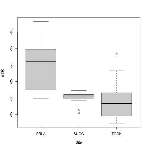
We see plants at Suggs and Toolik are quite low in 13C, with more
spread at Toolik than Suggs, and plants at Prairie Lake are relatively
enriched. Clearly the next question is what species these data represent.
But taxonomic data aren't present in the apl_plantExternalLabDataPerSample
table, they're in the apl_biomass table. We'll need to join the two
tables to get chemistry by taxon.
Every NEON data product has a Quick Start Guide (QSG), and for OS
products it includes a section describing how to join the tables in the
data product. Since it's a pdf file, loadByProduct() doesn't bring it in,
but you can view the Aquatic plant chemistry QSG on the
Product Details
page. The neonOS package uses the information from the QSGs to provide
an automated table-joining function, joinTableNEON().
apct <- joinTableNEON(apl_biomass,
            apl_plantExternalLabDataPerSample)
Using the merged data, now we can plot carbon isotope ratio for each taxon.
boxplot(analyteConcentration~scientificName,
        data=apct, subset=analyte=="d13C",
        xlab=NA, ylab="d13C",
        las=2, cex.axis=0.7)
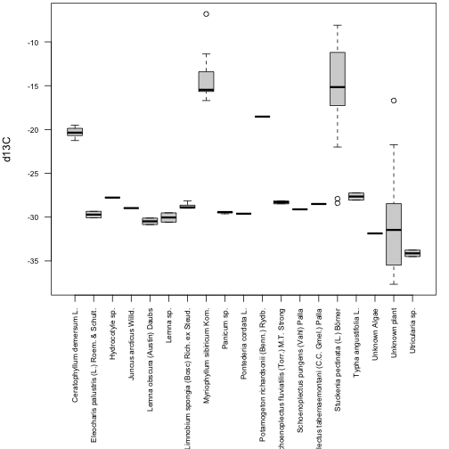
And now we can see most of the sampled plants have carbon isotope ratios around -30, with just two species accounting for most of the more enriched samples.
Download remote sensing data: byFileAOP() and byTileAOP()
Remote sensing data files are very large, so downloading them
can take a long time. byFileAOP() and byTileAOP() enable
easier programmatic downloads, but be aware it can take a very
long time to download large amounts of data.
Input options for the AOP functions are:
-
dpID: the data product ID, e.g. DP1.00002.001 -
site: the 4-letter code of a single site, e.g. HARV -
year: the 4-digit year to download -
savepath: the file path you want to download to; defaults to the working directory -
check.size: T or F: should the function pause before downloading data and warn you about the size of your download? Defaults to T; if you are using this function within a script or batch process you will want to set it to F. -
easting:byTileAOP()only. Vector of easting UTM coordinates whose corresponding tiles you want to download -
northing:byTileAOP()only. Vector of northing UTM coordinates whose corresponding tiles you want to download -
buffer:byTileAOP()only. Size in meters of buffer to include around coordinates when deciding which tiles to download
Here, we'll download one tile of Ecosystem structure (Canopy Height Model) (DP3.30015.001) from WREF in 2017.
byTileAOP("DP3.30015.001", site="WREF", year="2017", check.size = T,

          easting=580000, northing=5075000, savepath="~/Downloads")
In the directory indicated in savepath, you should now have a folder
named DP3.30015.001 with several nested subfolders, leading to a tif
file of a canopy height model tile.
Navigate data downloads: AOP
To work with AOP data, the best bet is the terra package.
It has functionality for most analyses you might want to do.
We'll use it to read in the tile we downloaded:
chm <- rast("~/Downloads/DP3.30015.001/neon-aop-products/2017/FullSite/D16/2017_WREF_1/L3/DiscreteLidar/CanopyHeightModelGtif/NEON_D16_WREF_DP3_580000_5075000_CHM.tif")
The terra package includes plotting functions:
plot(chm, col=topo.colors(6))
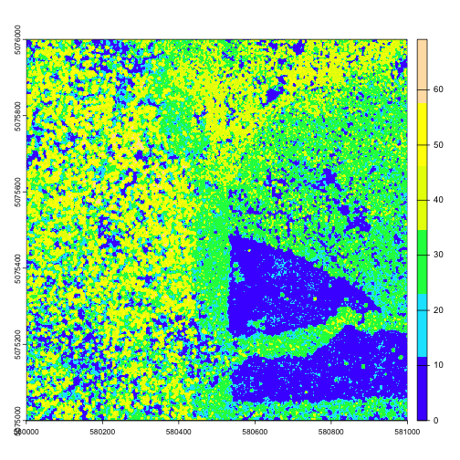
Now we can see canopy height across the downloaded tile; the tallest trees are over 60 meters, not surprising in the Pacific Northwest. There is a clearing or clear cut in the lower right quadrant.
Next steps
Now that you've learned the basics of downloading and understanding NEON data, where should you go to learn more? There are many more NEON tutorials to explore, including how to align remote sensing and ground-based measurements, a deep dive into the data quality flagging in the sensor data products, and much more. For a recommended suite of tutorials for new users, check out the Getting Started with NEON Data tutorial series.